User Guide
Introduction
The IonFrame class is the primary tool in the package. It represents the state of the ionosphere at a given
moment. IonFrame contains information about the date, instrument position, calculated electron
density and electron temperature in the instrument’s field of view. The raytrace() method
of the IonFrame
uses precalculated electron density to calculate the wave propagation trajectories through the ionosphere. In the
process, it also calculates the integrated absorption and emission of the ionosphere.
Initializing IonFrame
The IonFrame requires only two positional parameters: time of observation and position of the
instrument (basically, the center point of the model). The time should be specified using standard
datetime.datetime class. For example, let’s say we observe on November 7, 2020, at 13:00. In Python, it will look
like:
from datetime import datetime

dt = datetime(year=2020, month=11, day=7, hour=13)
# or
dt = datetime(2020, 11, 7, 13)
Note
The time in IonFrame must be specified in UTC.
The position of the instrument should be a tuple with three parameters: latitude in degrees, longitude in degrees, elevation above sea level in meters, For example:
pos = (45.5048, -73.5772, 0)
After that, the model is initialized by simply passing these two parameters to IonFrame:
from dionpy import IonFrame

frame = IonFrame(dt, pos)
print(frame)
Note
The electron density and temperature will be calculated at the moment of IonFrame initialization.
If you want to defer calculation, set IonFrame(..., autocalc=False) and later call IonFrame.calc()
to finish the calculation.
The printed output will be:
IonFrame instance
Date:   07 Nov 2020 13:00:00 UTC
Position:
        lat = 45.50 [deg]
        lon = -73.58 [deg]
        alt = 0.00 [m]
NSIDE:  64
IRI version:    2020
Use E-CHAIM:    False
Layer properties:
        Bottom height:  60 [km]
        Top height:     500 [km]
        N sublayers:    500
The output mentions some additional parameters we haven’t touched yet. Let’s discuss it now:
Parameter |
Explanation |
|---|---|
|
The |
|
The |
|
Setting |
|
Parameters |
|
The |
So, the initialization of the customized IonFrame can look something like this:
from dionpy import IonFrame
from datetime import datetime

dt = datetime(2020, 11, 7, 13)
pos = (45.5048, -73.5772, 0)
frame = IonFrame(dt, pos, nside=32, nlayers=200)
Raytracing within the frame
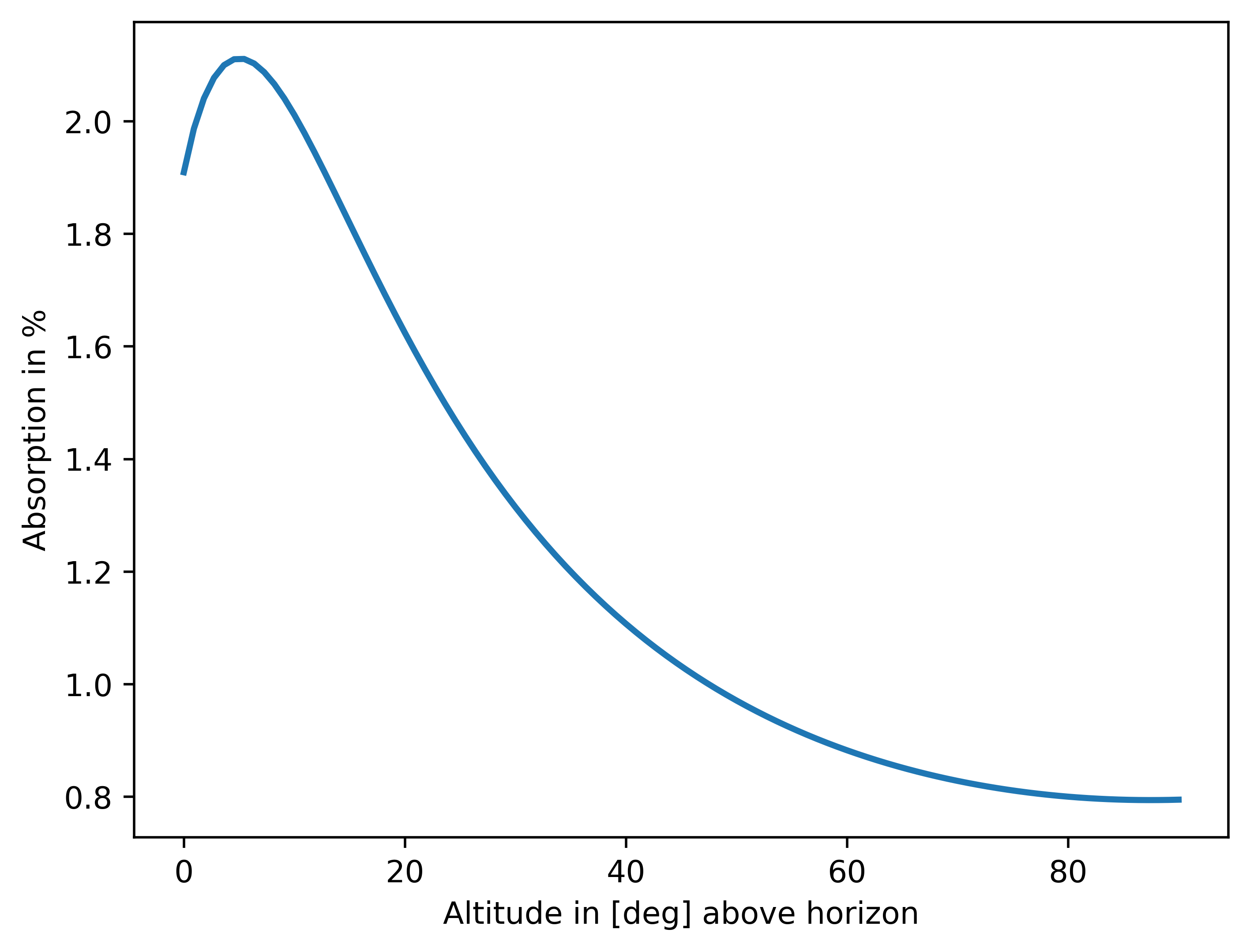
To perform the raytracing, one needs to specify two things: the ray’s initial direction and the wave’s frequency. While the frequency is a single float number in MHz, the direction is determined by coordinates in the horizontal coordinate system: altitude (also called elevation) and azimuth, both in degrees. Altitude and azimuth can be floats and numpy arrays of any dimensions. The raytracing output shape will match the coordinate array shape in the latter case. Consider the following example:
from dionpy import IonFrame
from datetime import datetime
import matplotlib.pyplot as plt

# Frame calculation
dt = datetime(2020, 11, 7, 13)
pos = (45.5048, -73.5772, 0)
frame = IonFrame(dt, pos, nside=32, nlayers=200)

freq = 40  # Specified in MHz
alt = np.linspace(0, 90, 100)
az = np.zeros(alt.shape)    # The azimuth is 0 for all specified altitudes

refr, atten, emiss = frame.raytrace(alt, az, freq)

# Plotting attenuation as an example
plt.plot(alt, (1 - atten) * 100, lw=2)
plt.ylabel("Absorption in %")
plt.xlabel("Altitude in [deg] above horizon")
plt.show()
Visualizing frames
IonFrame includes several pre-implemented methods to visualize the ionosphere’s state and the
raytracing results. These inlude: plot_ed(), plot_et(),
plot_atten(), plot_refr(), plot_emiss() and
plot_troprefr() (click on the name for more info). While these methods plot different data, they
all share a set of parameters listed below.
Parameter |
Explanation |
|---|---|
|
Title of the plot. |
|
Text label next to the colorbar. Most implemented methods override this parameter. Set
|
|
Bool indicating whether to include an additional text label. This label usually includes frame info - date/time, location and frequency of an observation. If set to None - no label is added. |
|
A tuple containing custom bottom and top limits for the colorbar. |
|
A path to save the plotted figure. Must also include the name of the file. If not specified - the figure will not be saved. |
|
Image resolution (when saving). |
|
A colormap to use. Can be a custom colormap or a string specifying existing matplotlib colormap. |
|
Formatter of numbers on the colorbar scale. |
|
A color to fill np.nan in the plot (default - black). |
|
A color to fill np.inf in the plot (default - white). |
|
Integer representing the difference between local time and UTC. If specified - local time is shown instead of UTC. |
|
If True - places the |
|
If True - the font size of labels is increased. |
|
If False - the colorbar is removed from the plot. |
|
If True - the position of the sun is plotted on top. Dashed line if the Sun is below horizon. |
Here are some examples.
from dionpy import IonFrame
from datetime import datetime
import matplotlib.pyplot as plt

dt = datetime(year=2022, month=7, day=17, hour=12, minute=0)
pos = (45.5048, -73.5772, 0)
frame = IonFrame(dt, pos, nlayers=200, nside=32)
freq = 40
frame.plot_atten(freq,
                 barlabel=r"Attenuation factor $f_a$",
                 cbformat="{x:.3f}",
                 plotlabel=None,
                 sunpos=True,
                 lfont=True)
plt.show()

In the picture above, the circle with the dot indicates the position of the sun in the sky (solid contour means above horizon; dashed - below horizon).
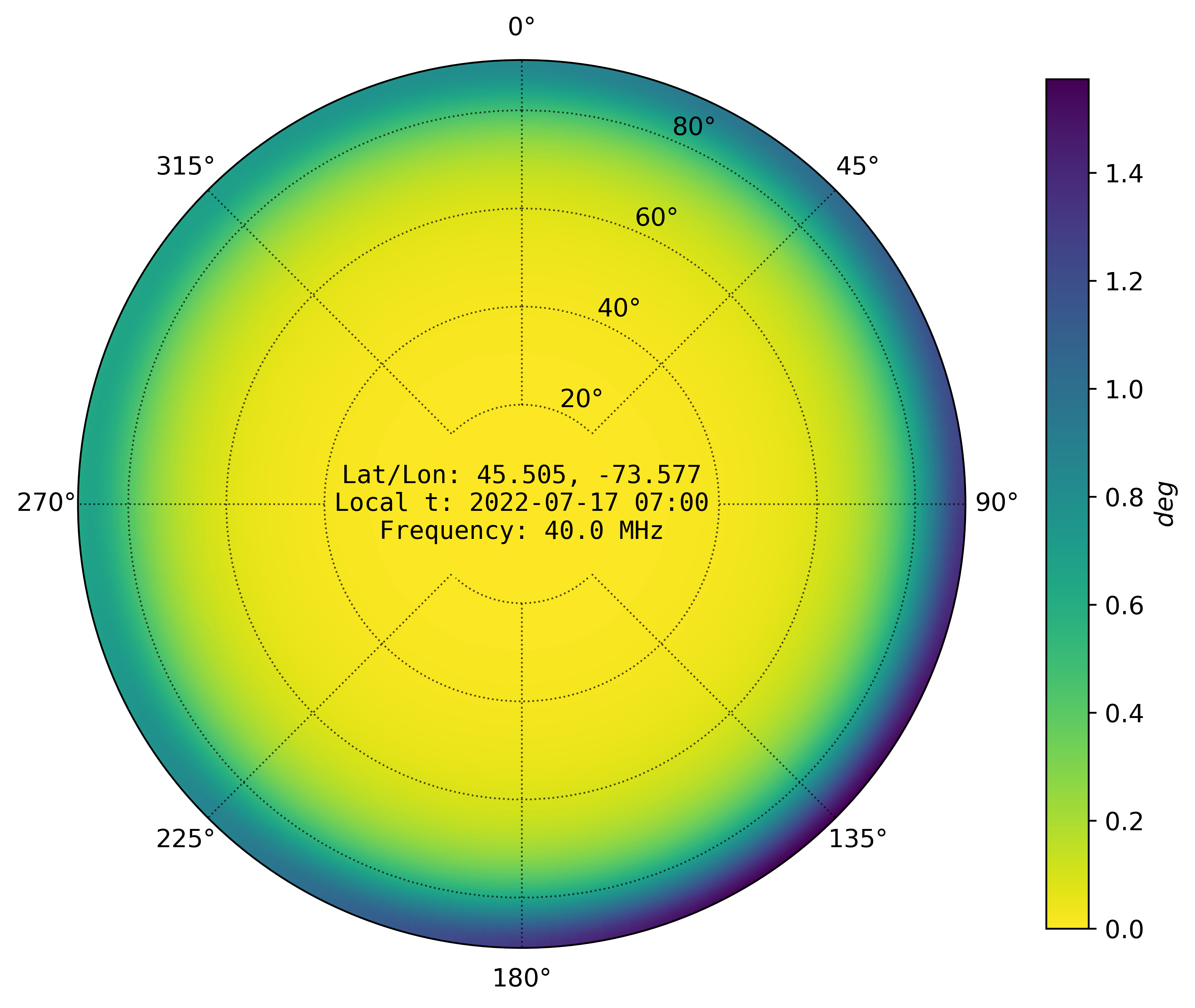
Using the same frame, let’s now plot refraction.
frame.plot_refr(freq,
                cinfo=True,
                cmap="viridis_r",
                local_time=-5)
plt.show()
Introducing IonModel
If you want to perform a continuous modelling of the ionosphere, generating an IonFrame for each time step
might be an overkill. On a small time scale (about several minutes) a linear interpolation between two IonFrames
gives a good approximation of the temporal evolution of the ionosphere. This interpolation is already implemented
within the IonModel class. IonModel is a collection of successive IonFrames
uniformly distributed in time. By using linear interpolation, one can calculate an IonFrame for any time within
the model range.
The initialization of IonModel is similar to IonFrame, except two time stamps
are required, which represent the start and the end times. Additional parameter - mpf (minutes per frame) -
controls the temporal resolution of the IonModel. For example, mpf=15 means that a new
IonFrame will be generated every 15 minutes.
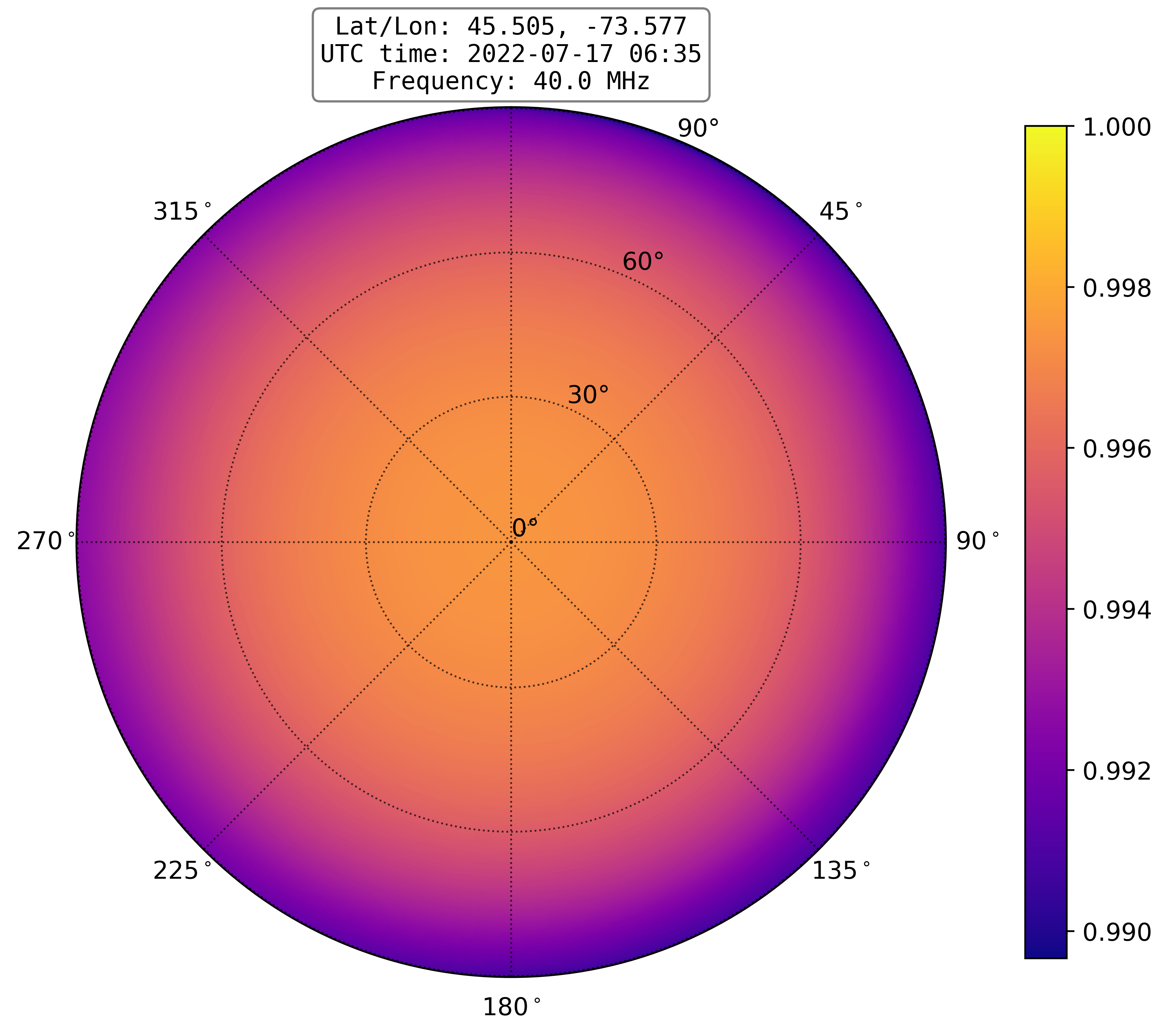
The interpolation is done using the at() method, which accepts a datetime object and returns
an IonFrame at the specified time. Here is an example.
from dionpy import IonModel
from datetime import datetime
import matplotlib.pyplot as plt

dt_start = datetime(year=2022, month=7, day=17, hour=6, minute=0)
dt_end = datetime(year=2022, month=7, day=17, hour=7, minute=0)
dt_middle = datetime(year=2022, month=7, day=17, hour=6, minute=35)
pos = (45.5048, -73.5772, 0)

model = IonModel(dt_start, dt_end, pos, mpf=10, nlayers=200, nside=32)
frame = model.at(dt_middle)

freq = 40
frame.plot_atten(freq)
plt.show()
The output will be:
Calculating time frames: 100%|██████████████████████████████████| 7/7 [00:09<00:00, 1.29s/it]
Saving frames and models
Calculating frames can take significant time, especially for greater-resolution grids. It takes even
more time for IonModels. In the last section’s example, the model calculation took 9 seconds. But
for longer models (say, several hours or days) it would be better to save the calculated model to
the disk and load it later. In dionpy, it is done with save() and load() methods.
These methods work both for IonFrame and ()
The save() method saves the whole model to the HDF file. It
requires specification of the path, including the name of the file. For example:
frame.save("frames/my_frame")
# or
model.save("models/my_model.h5")
# (specification of file extension is not necessary)
To load the saved model, use the load() class method of the appropriate class. For instance,
to load an IonFrame use
from dionpy import IonFrame
frame = IonFrame.load("frames/my_frame")
and for loading an IonModel use
from dionpy import IonModel
frame = IonModel.load("models/my_model")
Animating models
The IonModel also includes the animate() method, which allows the creation of animated
videos of the temporal evolution of specified parameters. The main parameters of the animate()
are:
Parameter |
Explanation |
|---|---|
|
Location of the output files. Defaults to the script execution directory (“./”). |
|
Frames per second. |
|
Total duration of the video in seconds. |
For example, let’s generate videos of attenuation and refraction for a period of one day. We will set the total duration to 10 seconds and fps to 20 frames/sec.
from dionpy import IonModel
from datetime import datetime

dt_start = datetime(year=2022, month=7, day=17)
dt_end = datetime(year=2022, month=7, day=18)
pos = (45.5048, -73.5772, 0)

model = IonModel(dt_start, dt_end, pos, mpf=30, nlayers=200, nside=32)

freq = 40
model.animate(freq=freq, target=["atten", "refr"], fps=20, duration=5, cinfo=True)
The output will be:
Calculating time frames: 100%|█████████████████████████████| 49/49 [01:03<00:00,  1.30s/it]
Animation making procedure started
Calculating data
Raytracing frames: 100%|███████████████████████████████████| 101/101 [00:35<00:00,  2.83it/s]
Rendering atten frames: 100%|██████████████████████████████| 101/101 [00:35<00:00,  2.84it/s]
Rendering atten animation: 100%|███████████████████████████| 100/100 [00:03<00:00, 33.24it/s]
Rendering refr frames: 100%|███████████████████████████████| 101/101 [00:33<00:00,  3.06it/s]
Rendering refr animation: 100%|████████████████████████████| 100/100 [00:02<00:00, 46.60it/s]
The generated attenuation video:
The generated refraction video: